| Unmasking the Noise: Masked and Denoising Autoencoders in Image Representation | |||
| Monica Chan | Frank Lee | Ivy Wu | |
| Final project for 6.7960, MIT | |||
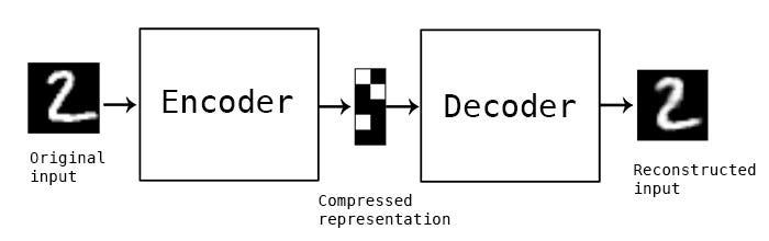
Figure 1. Autoencoder structure consisting of the encoder, latent space representation,
and decoder [7].
| Unmasking the Noise: Masked and Denoising Autoencoders in Image Representation | |||
| Monica Chan | Frank Lee | Ivy Wu | |
| Final project for 6.7960, MIT | |||
The rapid advancement of self-supervised learning (SSL) techniques has paved the way for more efficient and scalable machine learning models, particularly in the fields of computer vision and natural language processing. At the heart of many SSL frameworks is the autoencoder, a powerful tool for learning compact latent representations that capture the most salient features of the data and can be applied to downstream tasks like classification, clustering, and anomaly detection [2].
Building on this foundation, more sophisticated variants like denoising autoencoders (DAEs) and masked autoencoders (MAEs) have been introduced. Both types of autoencoders employ some form of input data alteration — whereas DAEs corrupt the image with noise, encouraging the model to focus on underlying patterns rather than superficial details, MAEs mask out random portions of the input and train the model to reconstruct the missing information, leveraging the context provided by unmasked regions. These modifications make DAEs and MAEs particularly effective in capturing more robust and meaningful representations, with applications across various domains.
Recent research has shown that MAEs often outperform DAEs in the field of computer vision, particularly on high-level semantic tasks such as image classification and semantic segmentation [1]. However, the reasons behind this superior performance remain an open question — the original MAE paper itself concludes with the hypothesis that the behavior "occurs by way of a rich hidden representation inside the MAE" and the hope that "this perspective will inspire future work" [4]. To address this, we examine the latent representations generated by each model type to uncover the key features and patterns they prioritize. Through this analysis, we aim to provide a deeper understanding of why MAEs excel in certain tasks and offer insights into optimizing both models for a broad range of applications.
Typical autoencoders aim to learn an efficient latent representation of the input data. The model consists of two main parts: the encoder that compresses the input image into the latent space and the decoder that reconstructs the original image.
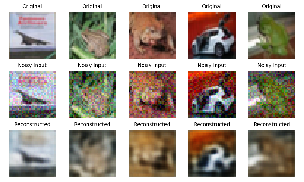
DAEs are designed to reconstruct an original image from noisy input data. During training, the model requires two sets of data: one with the original, clean images and another where random noise, typically Gaussian, is added. The DAE structure itself remains similar to a basic autoencoder, relying on convolutional layers to first compress the input image in the encoder and later reconstruct it through the decoder. In the forward pass, the model takes in the noisy image as input and calculates the loss between the final reconstruction and the original noise-less image. This encourages the model to focus on the true underlying features, rather than the noise introduced in the input [6].
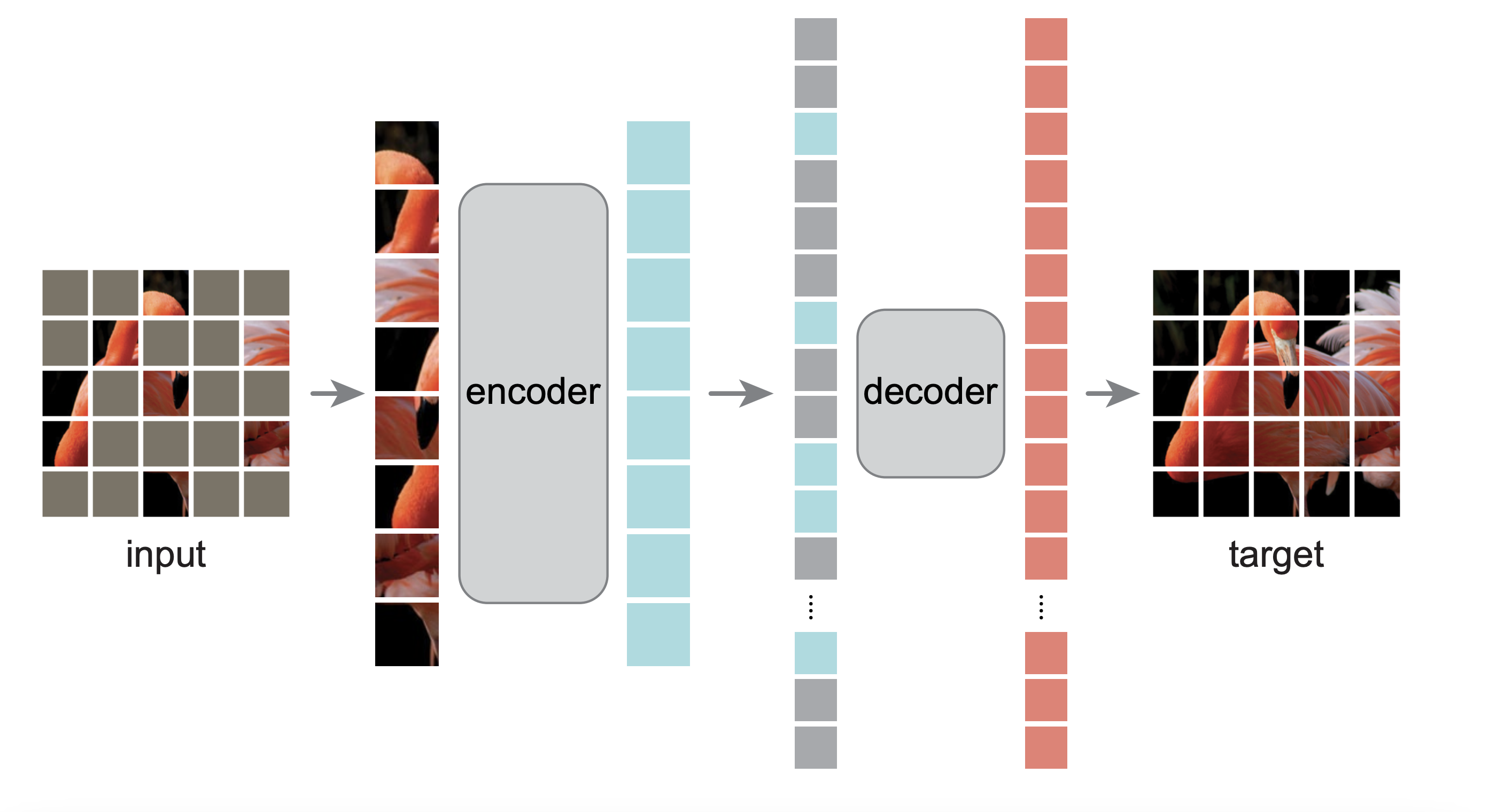
MAEs are a form of denoising autoencoders that aim to reconstruct a full image given only random patches of the original image. The researchers that developed MAEs were originally inspired by BERT, a language model that makes use of masked tokens. BERT will mask k% of the input sequence of words and learn to predict the masked words [3]. With the introduction of vision transformers that tokenize images into individual patches, this sort of masked prediction model can be applied to images instead of purely relying on convolutional operations.
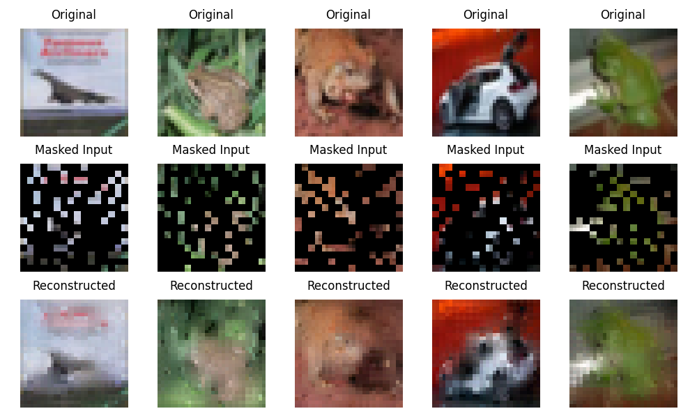
For a given input image, an MAE separates it into patches and randomly masks a certain percentage of them. The encoder operates only on the visible, unmasked patches, and it utilizes the self-attention mechanism of vision transformers (ViTs) to capture both local and global features from the unmasked patches. The resulting latent space consists of the embeddings of each of the unmasked patches. The decoder relies on these embeddings to reconstruct the masked patches before converting the patches back into the full image. Finally, loss between the original and reconstructed images is calculated for the masked areas alone.
After the initial pre-training phase, which focuses solely on minimizing the reconstruction loss, both DAEs and MAEs are fine-tuned for specific downstream tasks. For instance, in image classification, a classification head is attached to the encoder, where it is responsible for taking in the latent representations and producing class logits. The model's performance is then evaluated by computing the cross-entropy loss between the predicted class probabilities and the ground truth labels. This fine-tuning step allows the pretrained model to leverage its learned representations for accurate predictions on the specific task at hand.
Our group hypothesized that ViT-based MAEs may produce a more meaningful latent space compared to simpler, purely convolutional DAEs. Specifically, if we observe well-defined clusters in the latent space representations of inputs from the same image class, we can conclude that the MAE's latent space captures more semantic information about the actual input image.
To verify this hypothesis, we evaluated the performance of the MAE and DAE models on three downstream image classification tasks: one on the MNIST dataset, one on the CIFAR-10 dataset, and one on a color-jittered version of the CIFAR-10 dataset. For each of these experiments, we evaluated both models from the following angles:
All experiments were conducted using the same base architecture for the DAE, which utilized three convolutional layers for the encoder and three more for the decoder [11], and the MAE, which employed the original implementation from the MAE paper that can be found on Github [10]. Our only modification to the MAE architecture was the creation of a custom block class designed to return the attention mechanism if specified, enabling the visualization of attention maps. Additionally, each experiment built a wrapper around these base architectures to account for the specific characteristics of the datasets we were training on, ensuring the models were properly configured to handle the variations in input data size and task requirements. All reconstruction losses were calculated using a mean squared error (MSE) on the element-wise differences, and all classification losses were calculated using a cross-entropy loss.
Our group began the project by training a DAE and an MAE on the MNIST dataset, chosen for its simplicity and suitability for prototyping. The input to the models was a 28×28×1 tensor, representing image dimensions and a single grayscale channel. The MNIST dataset contains 60,000 training examples and 10,000 test examples, with each image paired with a label indicating the digit it represents [8].
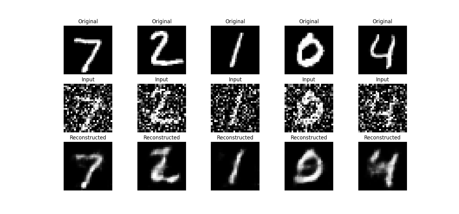
The DAE had a latent space size of 8x3x3 per image. It was trained for 20 epochs with a noise factor of 0.5 and optimized with an Adam optimizer with a learning rate of 0.001. For the downstream classification task, the classification head was composed of three linear layers interspersed with normalization, ReLU, and dropout layers that ultimately reduced the output to just 10 channels. The DAE encoder and classifier head were further fine-tuned for 20 epochs with a learning rate of 0.001, achieving a final test accuracy of 88.9%.
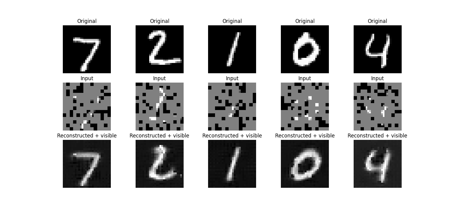
The MAE was trained with a patch size of 2 and a mask ratio of 0.75, resulting in a latent space size of 50x64, where 50 was the number of visible patches plus one for the CLS token. Like with the DAE, we employed an Adam optimizer with a learning rate of 0.001 to train the MAE for 20 epochs. The classification head was a simple linear layer that reduced the CLS token's latent representation to 10 channels, and, after fine-tuning, the overall model achieved a test accuracy of 92.86%.
In addition to the classification accuracies, we provide visualizations of the original, input, and reconstructed images for both the DAE and MAE below for human quality assessment.
The CIFAR-10 dataset consists of 60000 images, split into 50000 training images and 10000 testing images. Each 32x32x3 RGB image is labeled with one of ten classes: airplane, automobile, bird, cat, deer, dog, frog, horse, ship, or truck [9].
The DAE had a latent space of size 48x4x4 and was trained for 20 epochs with a noise factor of 0.1 and an Adam optimizer with a learning rate of 0.0003 and a weight decay of 1e-5. The encoder and classification head, which followed the same architecture as that of the DAE classification head from the MNIST experiment, were fine-tuned for 10 epochs, achieving a final classification accuracy of 48.67%.
The MAE had a latent space of size 65x192, where 192 was the chosen embedding dimension and 65 was the number of visible patches plus one for the CLS token, resulting from a patch size of 2 and a mask raito of 0.75. The MAE was pre-trained for 20 epochs with an Adam optimizer with a learning rate of 1e-4, and the encoder and classification head, a simple fully connected layer, were fine-tuned for 10 epochs, achieving a final accuracy of 74.78%.
The visualizations of the reconstructions from both models are shown below.
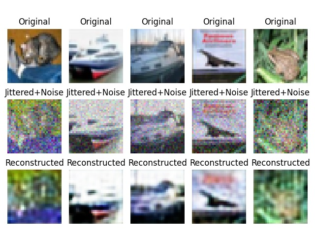
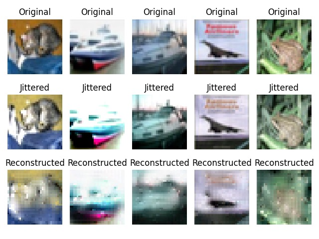
Our final experiment examined a known weakness highlighted in the original MAE paper: the reduced performance of MAE representations under color jittering.
During the pre-training phase, the CIFAR-10 input data underwent color jittering, where brightness, contrast, and saturation were adjusted by randomly chosen factors between 0.5 and 1.5, and hue was adjusted by factors between 0.9 and 1.1. Both the DAE architecture and MAE architecture were pre-trained for 20 epochs with a learning rate of 1e-4 and a weight decay of 1e-5. For both models, we employed a classification head that consisted of a simple fully connected layer. Using an optimizer that fine-tuned the existing MAE/DAE encoder with a learning rate of 1e-5 and trained the classification head with a learning rate of 1e-3, we found that the MAE classifier achieved a classification accuracy of 62.83%, while the DAE achieved a classification accuracy of 44.27%.
The images below show the reconstructions from both models.
| DAE (%) | MAE (%) | |
|---|---|---|
| MNIST | 88.9 | 92.86 |
| CIFAR-10 | 48.67 | 74.78 |
| Color-Jittered CIFAR-10 | 44.27 | 62.83 |
We analyze the outcomes of our three experiments, focusing on how the image accuracy metrics, latent space representation, and model weight distributions correlate with the overall classification accuracy that each model type achieved. Through these evaluations, we aim to provide a comprehensive understanding of how the architectures perform and adapt to varying dataset complexities.
Our hypothesis for why the MAE performs better was that the latent space contained more information that helped to distinguish the image. In order to test this theory, we decided to visualize the latent space for both the DAE and the MAE, using t-SNE to reduce the latent space dimensionality and plotting out an equal number of samples from each class [12].
For the MAE visualizations in particular, we applied t-SNE on and plotted only the CLS token. This is a placeholder token that is inserted at the beginning of the sequence right after generating the image patches and is designed to aggregate information from all of the other tokens throughout the encoding process. As a result, the CLS token is commonly used for downstream classification tasks, and in our project, we leverage it for classification as well. Since this is the only token used for classification, this is the only aspect that we are interested in visualizing.
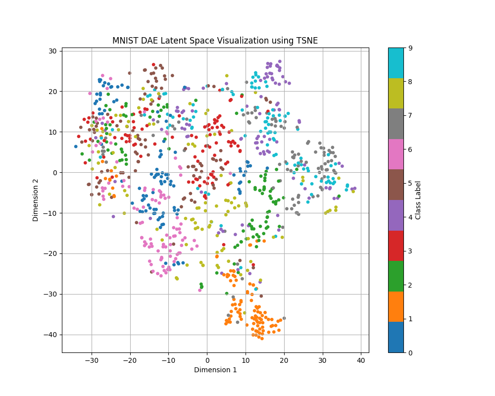
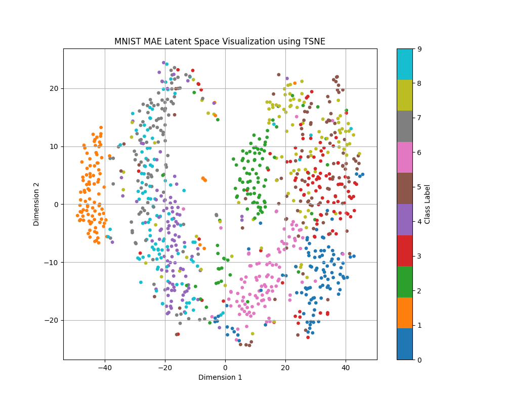
As shown in the visualizations, the MAE's latent space displays more distinct clusters according to the class labels, indicating that the MAE captures more semantic information about the image. The radius of the MAE clusters, calculated using the average Euclidean distance of the points from the center of the cluster, is also much smaller than that of the DAE, shown in the table below.
| Class | DAE Radius | MAE Radius |
|---|---|---|
| 0 | 10.3369 | 3.0710 |
| 1 | 8.5499 | 2.7798 |
| 2 | 9.9006 | 3.7947 |
| 3 | 8.5157 | 3.3625 |
| 4 | 10.6844 | 2.9421 |
| 5 | 8.8930 | 3.4431 |
| 6 | 9.8378 | 3.2537 |
| 7 | 9.0997 | 3.2447 |
| 8 | 9.9732 | 3.4379 |
| 9 | 8.6646 | 2.8606 |
The increased clustering effect in the MAE was also observed in the CIFAR-10 dataset across both the normal and color-jittered experiments, though not as pronounced. Unlike in the MNIST dataset, where there were separations between distinct clusters, the CIFAR-10 samples are much more mixed. This is likely due to the increased complexity of the dataset — images from the CIFAR-10 dataset are full-color RGB images, and there is much higher intra-class variability due to the nature of the categories. Furthermore, the backgrounds of the CIFAR-10 dataset are much more complex, compared to the fully black background of the MNIST dataset. The data gathered for the color-jittered CIFAR-10 experiment is included below, as the values of the normal CIFAR-10 experiment are quite similar.
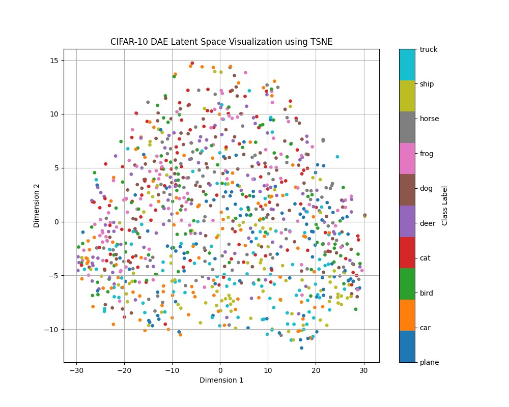
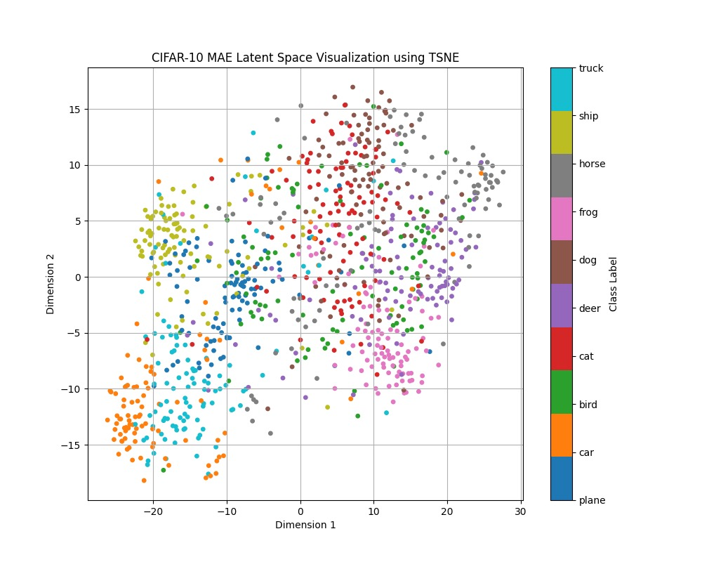
| Class | DAE Radius | MAE Radius |
|---|---|---|
| Plane | 20.8720 | 11.1166 |
| Car | 19.3819 | 9.2960 |
| Bird | 19.3067 | 11.9481 |
| Cat | 18.7238 | 11.7105 |
| Deer | 15.1067 | 12.0574 |
| Dog | 19.2490 | 11.6463 |
| Frog | 14.4154 | 10.1000 |
| Horse | 19.2148 | 11.0689 |
| Ship | 19.6614 | 10.5390 |
| Truck | 19.4636 | 9.5047 |
Across all experiments, the MAE outperformed the DAE in terms of clustering in the latent space. Each of the classes exhibited much tighter clusters, suggesting that the MAE's high classification accuracy is in part due to its discriminitive and semantically meaningful representations. With these tighter clusters, it becomes much easier for a classification head to learn the boundaries between classes.
For the DAEs, we generate saliency maps that measure how sensitive the latent representations are to perturbations in the input. For each value in the latent space, we calculate the gradients with respect to each pixel in the input image, combining these values per-pixel in order to measure each pixel's overall contribution to the latent representation. These contributions are then normalized to the [0, 1] range and displayed as a heatmap, with darker colors indicating lower impact and brighter colors indicating higher impact.
For the MAEs, we generate attention maps that indicate which patches the ViT encoder focused the most on during the forward pass. This is done by taking the attention weights from the ViT's last layer and multiplying these values against the patched masked image, creating one map per attention head. The resulting heatmaps are normalized to the [0, 1] range and displayed, following the same pattern where brighter colors indicate higher attention. An example for both the saliency and attention maps for the MNIST dataset is shown below.
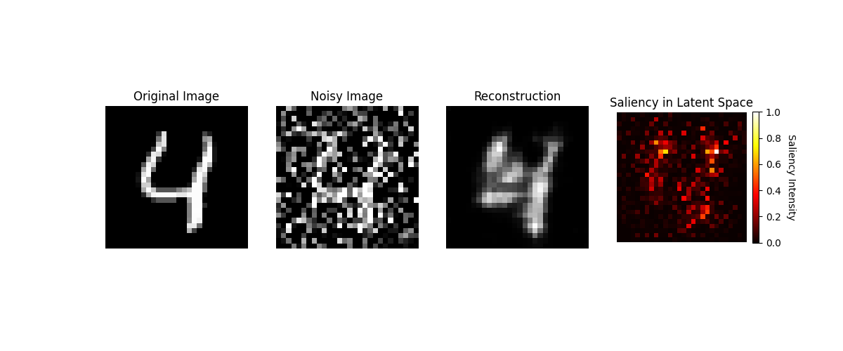
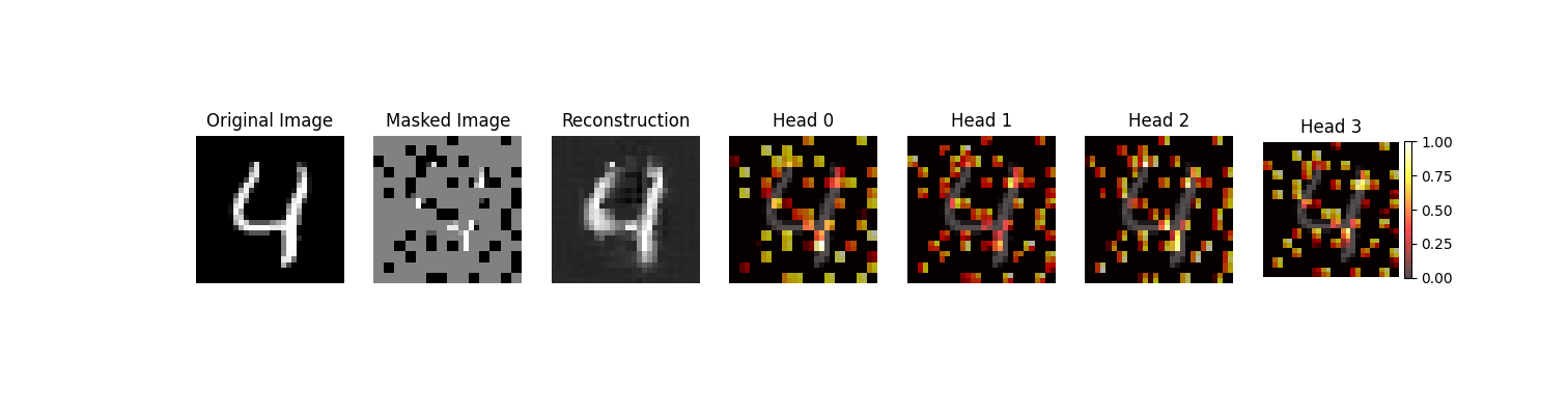
These maps demonstrate that the MAEs have a greater proportion of high-attention patches than the amount of high-saliency pixels in the DAEs, an effect that is again more pronounced in the MNIST than the CIFAR-10 dataset. This highlights the MAEs' ability to focus on semantically important regions of an image, as the targeted attention facilitates the encoding of meaningful features. On the contrary, the DAEs' large regions of low- to medium-saliency values result in the distribution of focus, likely due to the denoising process, and may lead to the model capturing less relevant details and making them less effective in downstream tasks.
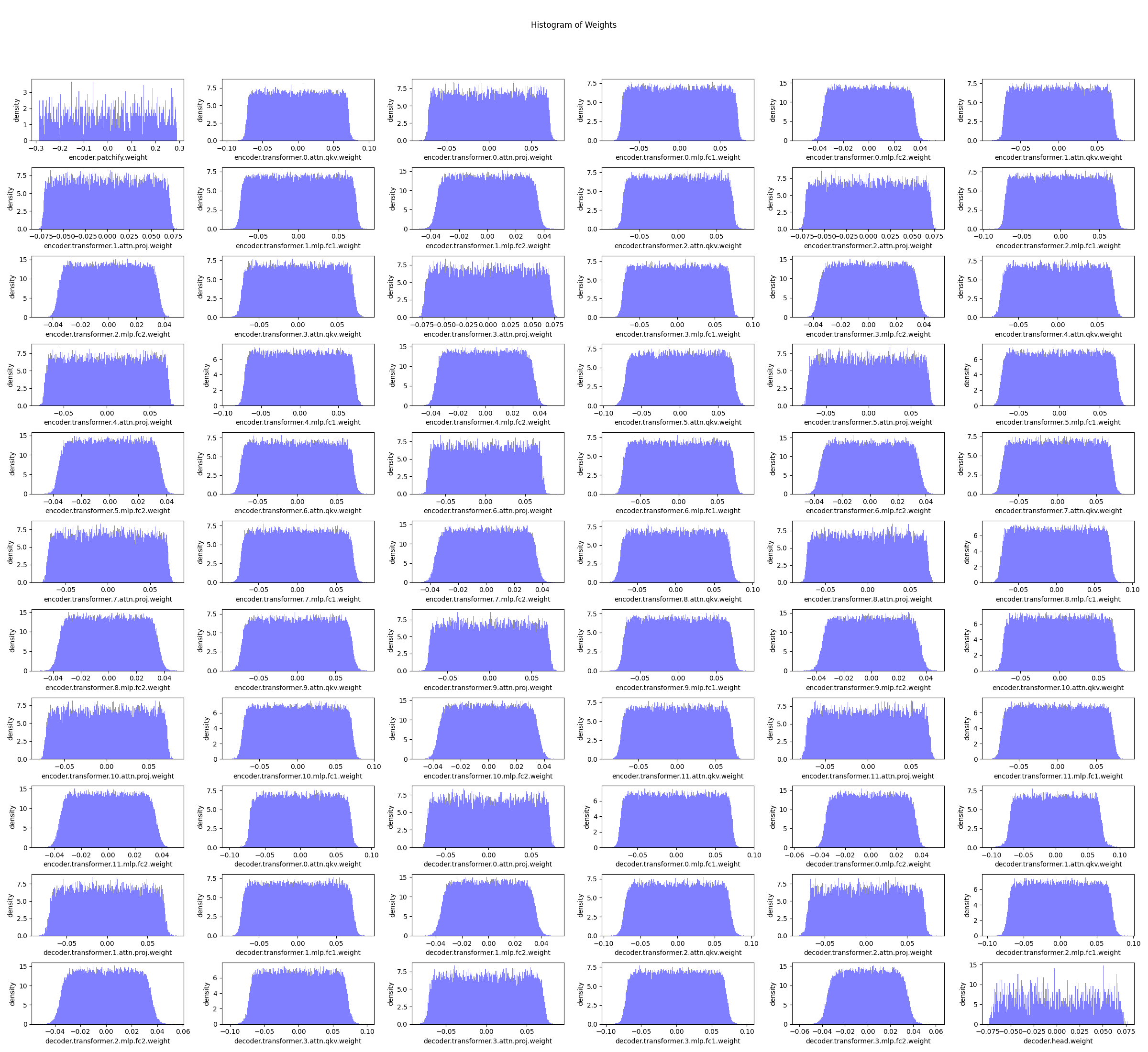
For each experiment, we plotted the weight distributions of each layer, ignoring normalization layers and the bias terms, of the DAE and the MAE models. An example of this distribution is shown below for the CIFAR-10 dataset.
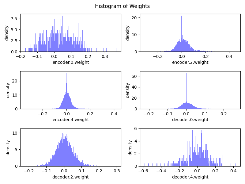
Across all experiments, including the color-jittered CIFAR-10 dataset, the weight distributions of the MAE and DAE follow the same pattern, revealing significant differences in how these models utilize their parameters. The DAE’s weights follow a Gaussian-like distribution and are heavily concentrated near zero, indicating that many neurons contribute minimally to the model's learning process. This sparsity suggests inefficiencies, as the DAE may overemphasize low-level details required for denoising, limiting its ability to extract high-level features essential for tasks like classification.
In contrast, the MAE exhibits a more evenly distributed weight range with fewer extreme values, reflecting more balanced and effective parameter utilization. This distribution allows the MAE to encode richer semantic features in its latent space, as evidenced by the tighter clustering of inputs from the same class in our latent space visualizations. Additionally, the MAE's weight characteristics likely enhance its stability and adaptability, contributing to its superior performance on the MNIST and CIFAR-10 datasets.
Across all experiments, contrary to our expectations due to the richer hidden representation of the MAE models, the DAE outperformed the MAE consistently in terms of PSNR and SSIM metrics, achieving higher values in both. A sample output calculation is shown below for the CIFAR-10 dataset.
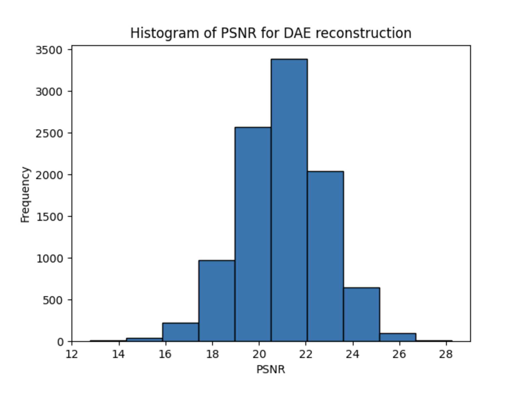
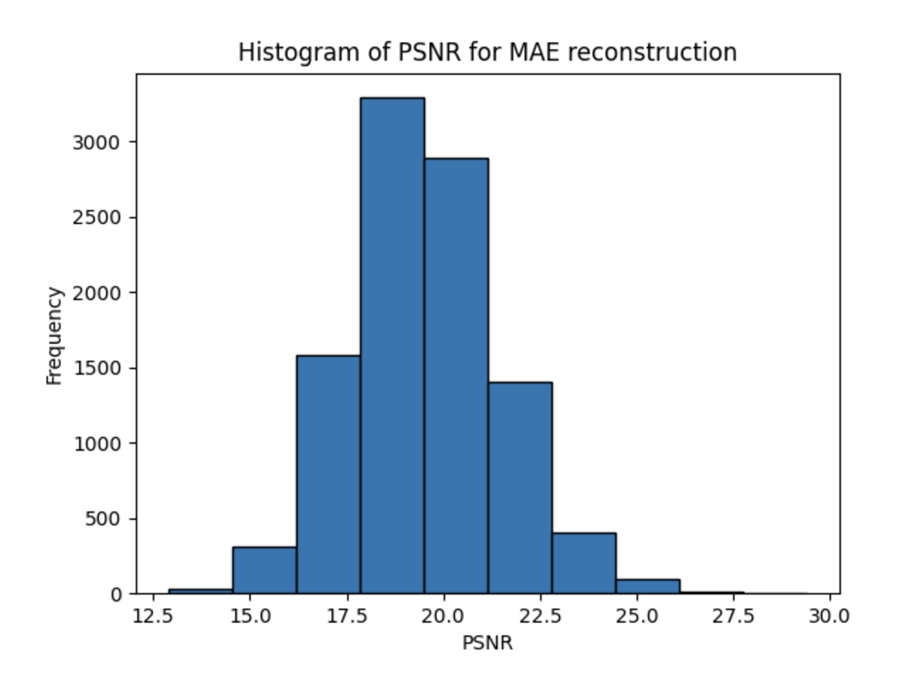
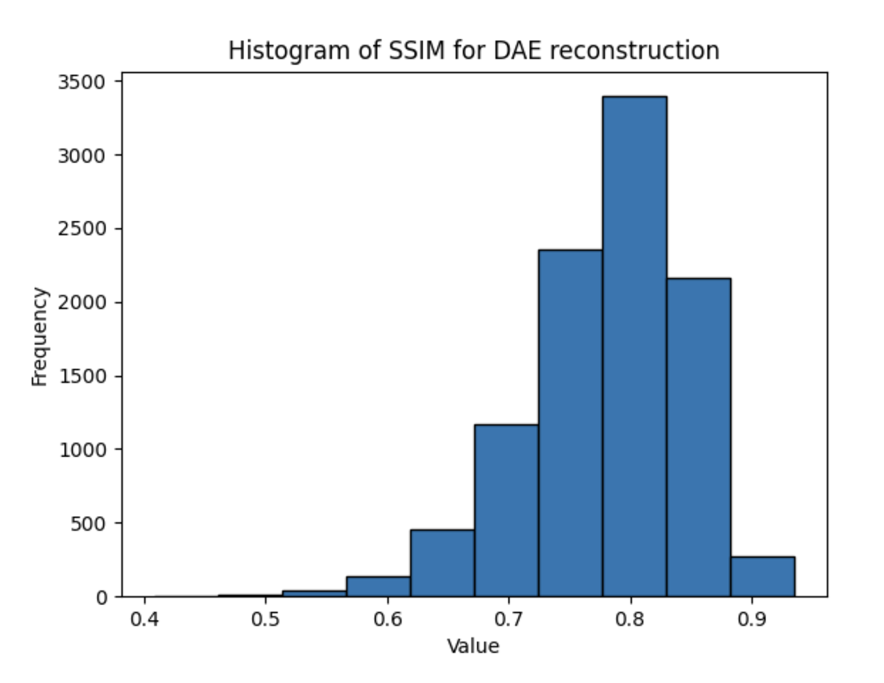
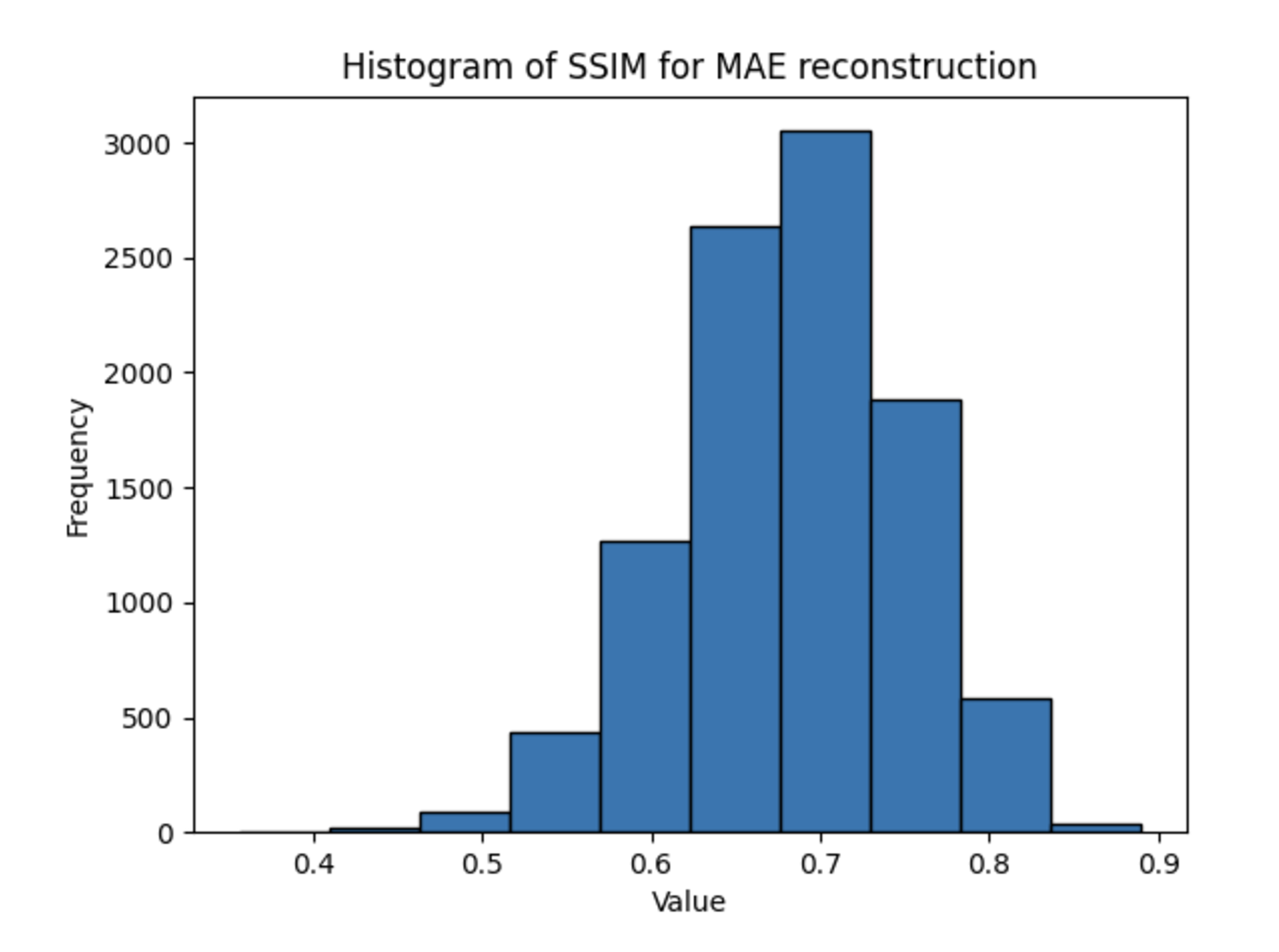
The PSNR and SSIM metrics for each experiment are shown below.
| DAE - PSNR | MAE - PSNR | DAE - SSIM | MAE - SSIM | |
|---|---|---|---|---|
| MNIST | 15.93 | 14.09 | 0.69 | 0.26 |
| CIFAR-10 | 20.9 | 19.2 | 0.79 | 0.69 |
| Color-Jittered CIFAR-10 | 24.01 | 21.38 | 0.78 | 0.69 |
One reason for these discrepancies may be the fact that the architectures take inherently different inputs: the MAE’s masked input may be a harder input to reconstruct, even if the weights learned when creating a latent representation are more useful for downstream tasks. While this addresses the superiority of the DAE in terms of PSNR, which measure purely per-pixel reconstruction accuracy, it cannot fully explain the better performance of the DAE in terms of SSIM, the metric for structural information. One explanation for this could be the small patch sizes used for the MAE training — each patch consists of only 4 pixels, limiting the structural information present.
To summarize our findings from each experiment:
The results provide valuable insights into the MAE's ability to outperform DAEs on high-level image classification tasks while shedding light on the underlying factors that enable its performance. The MAE demonstrated resilience to color-jittering, maintaining high classification accuracy and well-defined latent space clustering, even under input distortions. This robustness highlights the model's ability to capture meaningful semantic features, which are crucial for classification tasks. However, the lower PSNR and SSIM scores observed for the MAE reflect its trade-off in reconstruction quality, likely due to the limited information available in the masked inputs and the use of small patch sizes (2x2).
These findings reinforce the MAE's strength in tasks that prioritize semantic understanding over pixel-level accuracy. Future work could explore training MAEs on larger, more compute-intensive datasets, allowing for larger patch sizes that might improve both semantic and structural feature extraction. Additionally, further investigation into how the MAE mitigates distortions like color-jittering could inform improvements in robustness and generalization for other high-level tasks.
All code utilized for this project can be found on our Github repository.